RdistNN is an R package for conditional average treatment effects (CATE) and nonparametric regression using distributional nearest-neighbor (DNN) weights. It provides local estimates, delete-1 jackknife standard errors, weight and overlap diagnostics, and optional ggplot2 visualizations.
The initial public release focuses on cate_dnn(), np_dnn(), and the DNN weights and tuning tools supporting these workflows. Nuisance predictions for CATE are supplied by the user. All PLQR functionality is experimental, including its scores, demo data, inference methods, and plotting helpers. Local IV-GMM is also experimental; advanced extensions remain available in the reference documentation.
The package accompanies Orthogonal Inference for Conditional Z-Estimation without Cross-Fitting. See the documentation and Jakob Juergens’s website for project context.
Installation
Install release 0.1.0 from GitHub (R 4.1.0 or newer):
install.packages("pak")  # once
pak::pak("JakobJuergens/RdistNN@v0.1.0")
The v0.1.0 release also provides RdistNN_0.1.0.tar.gz with built HTML vignettes and a SHA256SUMS file. After installing Rcpp, install that source asset directly:
install.packages("Rcpp")  # once
install.packages(
  "https://github.com/JakobJuergens/RdistNN/releases/download/v0.1.0/RdistNN_0.1.0.tar.gz",
  repos = NULL, type = "source"
)
For the current development version, use pak::pak("JakobJuergens/RdistNN").
This installs from source and requires a C++17 toolchain and Rcpp. Use Rtools matching your R version on Windows, Xcode command line tools on macOS, or an R-compatible C++ compiler on Linux. OpenMP is optional; supported kernels run serially when R’s toolchain does not supply OpenMP flags.
The online guides are available independently of installation. To include local HTML vignettes, use:
install.packages("remotes")  # once
remotes::install_github("JakobJuergens/RdistNN", ref = "v0.1.0", build_vignettes = TRUE)
vignette("getting-started", package = "RdistNN")
Conditional average treatment effects
This example uses simulated data and oracle nuisance values to show the interface. For an application, replace these columns with your estimated conditional outcome means and treatment propensities.
library(RdistNN)

demo <- cate_demo_data(n = 180, p = 2, design = "hetero", seed = 1)
df <- demo$data
df$m1_oracle <- df$m0_oracle + df$tau_oracle

fit_cate <- cate_dnn(
  data = df, x_cols = c("X1", "X2"),
  y_col = "Y", t_col = "D",
  m0_col = "m0_oracle", m1_col = "m1_oracle", e_col = "e_oracle",
  x0 = c(0, 0), k = 1L, se = TRUE,
  return = c("W", "psi", "nuisance")
)

summary(fit_cate)
#> <summary.cate_result>
#>   targets: 1
#>          estimate std.error statistic p.value conf.low conf.high
#> target_1   0.4527    0.2607     1.737 0.08242 -0.05817    0.9636
confint(fit_cate)
#>             conf.low conf.high
#> target_1 -0.05817257 0.9636003
predict(fit_cate, x0 = c(0.2, -0.1), interval = "confidence")
#>            fit       lwr      upr
#> [1,] 0.7890503 0.4451826 1.132918
The matrix interface accepts an externally constructed pseudo-outcome: cate_dnn(X = X, x0 = x0, pseudo_outcome = psi). The getting-started guide shows both input formats and how to inspect local overlap.
CATE inference conditions
Neyman orthogonality controls first-order population nuisance drift. Valid full-sample nuisance reuse additionally requires the nuisance-rate and full-state stability conditions in the paper. cate_dnn() computes the estimator and jackknife procedure; it cannot establish those conditions for an arbitrary learner. Oracle, out-of-fold, and full-sample predictions can be supplied, but each inferential interpretation needs the corresponding assumptions, including overlap and localization bias control.
For nuisance-based AIPW and Robinson scores, supplied propensities must be finite and lie in [0, 1]; they are clipped to [clip, 1 - clip], with clip = 1e-8 by default. Clipping does not establish overlap. Supplied pseudo-outcomes are used unchanged. Reported intervals are pointwise, and do not provide simultaneous coverage of an entire covariate profile.
Nonparametric regression
demo_np <- np_demo_data(n = 180, p = 2, design = "sinusoidal", seed = 2)
fit_np <- np_dnn(
  data = demo_np$data, x_cols = c("X1", "X2"), y_col = "Y",
  x0 = c(0, 0), k = 1L, se = TRUE, return = c("W", "dx", "ess")
)

fit_np$mu
#> [1] 0.03318309
fit_np$se
#> [1] 0.1328814
diagnostics(fit_np)[, c("target_id", "n_eff", "weighted_mean_y")]
#> <dnn_diagnostics>
#>   targets: 1
#>   n_eff  : min=17.5249, median=17.5249, max=17.5249
#>   dist   : available for 0/1 target(s)
For matrices, use np_dnn(X = X, x0 = x0, Y = y). Regression results expose mu and se directly; CATE additionally provides summary(), confint(), and predict() methods. Both workflows support diagnostics(), plot_data_estimates(), and optional plot() methods.
Two-scale regression is available through np_tdnn() with explicit s1 < s2 (s2 < n for jackknife standard errors). Its signed weights and additional smoothness requirements are explained in the getting-started guide and ?np_tdnn; plot_tdnn_scales() compares the component scales.
Localization and tuning
With k = 1 and no explicit s, the default is s = floor(0.4 * n^((p + 1)/(p + 2))). Here s is the subsample order: increasing it concentrates weights closer to the target. Exact DNN weights average over size-s subsamples, using the full rank permutation, with support through rank n - s + k. The optional neighbors extra reports the first k neighbors, rather than the full weight support.
Use tuning = tuning_dnn_paper() to specify the paper’s rule, or tuning_mode = "grid" to compare its sensitivity grid lambda = c(0.3, 0.4, 0.5, 0.75). candidate_fit() and plot_tuning() inspect the stored candidates. The manuscript derivations use k = 1; larger fixed k values are implementation-supported generalizations.
Delete-1 standard errors require s < n. jackknife = "fast" uses cached ranks; "loo" recomputes leave-one-out weights. Set se = FALSE to skip uncertainty calculations. Weight ESS and overlap diagnostics help describe local support; they do not verify the assumptions needed for inference.
Visualizing CATE
If ggplot2 is installed, plot(fit) displays estimates with pointwise jackknife confidence bounds. This profile holds the second covariate at zero and again uses oracle nuisance inputs.
library(RdistNN)

set.seed(42)
n <- 1000
X <- cbind(X1 = runif(n, -2, 2), X2 = rnorm(n))
e <- plogis(0.4 * X[, "X1"])                    # oracle propensity
tau <- 1 + sin(X[, "X1"])                       # true CATE along X1
m0 <- X[, "X1"] - 0.5 * X[, "X2"]               # oracle control mean
treat <- as.integer(runif(n) < e)
Y <- m0 + treat * tau + rnorm(n, sd = 0.5)

df <- data.frame(X, T = treat, Y = Y, e = e, m0 = m0, m1 = m0 + tau)
X0 <- cbind(X1 = seq(-1.8, 1.8, length.out = 21), X2 = 0)

fit <- cate_dnn(
  data = df, x_cols = c("X1", "X2"), y_col = "Y", t_col = "T",
  e_col = "e", m0_col = "m0", m1_col = "m1",
  X0 = X0, k = 1L, se = TRUE, jackknife = "fast"
)

plot(fit)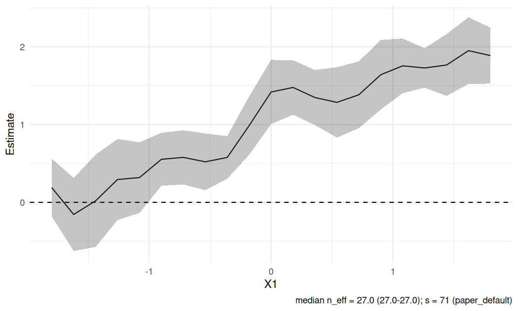
Use plot_weights() for weight concentration, plot_overlap() for local treatment support, and plot_influence() for score contributions. plot_dashboard() additionally requires patchwork. The visualization guide shows the available panels and their underlying data extractors.
Documentation and release scope
| Workflow | Entry points | Status |
|---|---|---|
| CATE |
cate_dnn(), CATE methods and diagnostics |
Release focus |
| Nonparametric regression |
np_dnn(), np_tdnn(), diagnostics and plots |
Release focus; TDNN uses signed weights |
| Localization | DNN weights, distances, tuning | Supports the main workflows |
| Affine paper replication | Installed paper-replication/affine scripts |
Current affine simulations, SIPP, and accepted evidence |
| Synthetic CATE benchmarks |
sim_cate_*, summarise_sim_results()
|
General simulation tools |
| PLQR |
plqr_dnn(), PLQR scores, helpers and methods |
Experimental; evaluates moments at supplied coefficients, without root solving |
| Local IV-GMM |
gmm_dnn(), sim_iv_*
|
Experimental companion work |
| Extensions | Registries, generalized U-statistic utilities | Advanced reference material |
Start with Getting started, then read notation and conventions, diagnostics, and tuning. The affine paper replication guide covers the current bounded simulations, SIPP application, and regeneration of accepted manuscript tables and figures. Validation runs are labeled separately from production. Locate the installed bundle with system.file("paper-replication/affine", package = "RdistNN").
With local vignettes installed, open the symbol guide with vignette("notation-and-conventions", package = "RdistNN").
Development and help
Report issues with a minimal reproducible example through the issue tracker. See CONTRIBUTING.md for local checks and RELEASING.md for source packaging and publication instructions. The package is licensed under GPL version 3 or later.
Supported R algorithmic fallbacks can be selected with options(RdistNN.use_compiled = FALSE); source installation still requires a compiler. Cross-platform CI covers Linux, Windows, and both macOS architectures. Edit README.Rmd and regenerate with devtools::build_readme().