Getting started: CATE and regression

The initial RdistNN release focuses on conditional average treatment effects and nonparametric regression with distributional nearest-neighbor (DNN) weights. Both estimators accept numeric matrices or data frames, including tibbles through the data-frame interface. Inputs must be finite and complete; choose covariate columns explicitly and supply one of x0 (one target) or X0 (one target per row).

PLQR and local IV-GMM are experimental. Their reference material is available for research use, but they are outside the supported workflow focus of this release. PLQR evaluates moments at supplied coefficients; it does not solve for target-specific coefficients.

Conditional average treatment effects

For binary treatment D, the AIPW inputs are outcome Y, control and treated conditional means m0 and m1, and propensity e. Nuisance fitting is external to the package. This simulation supplies oracle nuisances so that the example demonstrates localization without choosing a nuisance learner.

demo_cate <- cate_demo_data(n = 180, p = 2, design = "hetero", seed = 1)
df <- demo_cate$data
df$m1_oracle <- df$m0_oracle + df$tau_oracle

fit_cate <- cate_dnn(
  data = df, x_cols = c("X1", "X2"), y_col = "Y", t_col = "D",
  m0_col = "m0_oracle", m1_col = "m1_oracle", e_col = "e_oracle",
  x0 = c(0, 0), k = 1L, se = TRUE,
  return = c("W", "psi", "nuisance", "dx")
)

summary(fit_cate)
#> <summary.cate_result>
#>   targets: 1
#>          estimate std.error statistic p.value conf.low conf.high
#> target_1   0.4527    0.2607     1.737 0.08242 -0.05817    0.9636
confint(fit_cate)
#>             conf.low conf.high
#> target_1 -0.05817257 0.9636003
predict(fit_cate, x0 = c(0.2, -0.1), interval = "confidence")
#>            fit       lwr      upr
#> [1,] 0.7890503 0.4451826 1.132918

fit_cate$tau contains the estimates and fit_cate$se contains their jackknife standard errors. confint() returns pointwise normal intervals; it does not provide a simultaneous confidence band for a profile.

If you already have an observation-level pseudo-outcome, pass it directly. Here we reuse the oracle AIPW scores retained by the preceding fit:

X <- as.matrix(df[c("X1", "X2")])
fit_cate_matrix <- cate_dnn(
  X = X, x0 = c(0, 0), pseudo_outcome = fit_cate$psi, k = 1L
)

c(data_frame = fit_cate$tau, matrix = fit_cate_matrix$tau)
#> data_frame     matrix 
#>  0.4527139  0.4527139

The data-frame pathway also accepts pseudo_outcome, or a Robinson-form score via y_col, t_col, m_col, and e_col. See ?cate_dnn for the complete input contract. Preserve the same observation order for every nuisance or pseudo-outcome vector.

Interpreting CATE inference

Orthogonality controls first-order population nuisance drift. Valid nuisance reuse on the full estimation sample additionally requires the nuisance-rate and full-state stability conditions in the accompanying paper. The package cannot establish those conditions for an arbitrary learner. Out-of-fold predictions are also accepted, but using them does not by itself establish all conditions needed for local inference. Overlap and localization bias control remain necessary.

Raw supplied propensities must lie in [0, 1] and are clipped to [clip, 1 - clip] with clip = 1e-8 by default. Diagnostics use the clipped values. Clipping does not create local treatment support, and a supplied pseudo-outcome is used unchanged.

Inspect local weight concentration and treated/control mass:

d_cate <- diagnostics(fit_cate)
d_cate[, c("target_id", "n_eff", "treated_mass", "control_mass")]
#> <dnn_diagnostics>
#>   targets: 1
#>   n_eff  : min=17.5249, median=17.5249, max=17.5249
#>   dist   : available for 0/1 target(s)

Diagnostics describe the realized sample near a target; they are not a test of the paper’s assumptions. Keep "W" in return for weight diagnostics, "dx" for distance-radius summaries, and "nuisance" for explicit nuisance inspection. For CATE overlap, the hidden fitted state retains treatment and propensity inputs when these were supplied.

Nonparametric regression

np_dnn() estimates a conditional mean by averaging outcomes with DNN weights. Its result exposes mu and se directly. The explicit CATE summary(), confint(), and predict() methods do not apply to np_result.

demo_np <- np_demo_data(n = 160, p = 2, design = "sinusoidal", seed = 2)
fit_np <- np_dnn(
  data = demo_np$data, x_cols = c("X1", "X2"), y_col = "Y",
  X0 = rbind(c(0, 0), c(0.5, 0)), k = 1L, se = TRUE,
  return = c("W", "dx", "ess")
)

# Normal pointwise intervals from the stored jackknife standard errors.
plot_data_estimates(fit_np)[, c("target_id", "estimate", "se", "ci_lower", "ci_upper")]
#>   target_id    estimate        se    ci_lower  ci_upper
#> 1         1 -0.08841632 0.1517981 -0.38593504 0.2091024
#> 2         2  0.24768566 0.1328475 -0.01269067 0.5080620
diagnostics(fit_np)[, c("target_id", "n_eff", "weighted_mean_y")]
#> <dnn_diagnostics>
#>   targets: 2
#>   n_eff  : min=17.3549, median=17.3549, max=17.3549
#>   dist   : available for 0/2 target(s)

Use uppercase Y for the matrix interface:

fit_np_matrix <- np_dnn(
  X = as.matrix(demo_np$data[c("X1", "X2")]),
  Y = demo_np$data$Y, x0 = c(0, 0), k = 1L
)
fit_np_matrix$mu
#> [1] -0.08841632

To estimate at new regression targets, call np_dnn() with those targets. The intervals above need the regression assumptions and localization bias control; the jackknife alone does not remove smoothing bias.

Two-scale nonparametric regression

np_tdnn() provides the existing two-scale DNN regression alternative. Supply orders s1 < s2; delete-1 standard errors additionally require s2 < n. Its weights sum to one but can be negative, so positive-weight CATE overlap interpretations do not carry over. Its bias-correction interpretation needs the additional smoothness conditions described in ?np_tdnn.

fit_tdnn <- np_tdnn(
  data = demo_np$data, x_cols = c("X1", "X2"), y_col = "Y",
  x0 = c(0, 0), s1 = 8L, s2 = 16L, se = TRUE
)
c(estimate = fit_tdnn$mu, standard_error = fit_tdnn$se)
#>       estimate standard_error 
#>     -0.2026243      0.1984072

The matrix interface uses X, Y, and x0/X0, as for np_dnn(). Use plot_tdnn_scales() to compare the two scales when ggplot2 is available. The single-scale paper tuning rule discussed below applies to np_dnn() and cate_dnn(); choose the two TDNN orders explicitly.

Choosing localization and uncertainty settings

The defaults use exact DNN weights and k = 1. Unless s or tuning is supplied, the subsample order is s = floor(0.4 * n^((p + 1)/(p + 2))), where p is the covariate dimension. Larger s concentrates more weight near the target. The written manuscript derivations use k = 1; larger fixed k is supported in the implementation.

The order s is not a count of observations retained in a nearest-neighbor truncation. Exact weights use the full rank permutation and have support through rank n - s + k (n - s + 1 for k = 1). The optional neighbors extra reports the first k neighbors, rather than the full weight support.

For sensitivity analysis, compare the paper’s candidate orders without changing the primary result:

fit_grid <- np_dnn(
  data = demo_np$data, x_cols = c("X1", "X2"), y_col = "Y",
  x0 = c(0, 0), tuning_mode = "grid", se = FALSE
)
fit_grid$tuning_grid$candidates
#>   candidate_id computed_key is_default feasible reason status lambda  s
#> 1   lambda_0p3         s_13      FALSE     TRUE     ok     ok   0.30 13
#> 2   lambda_0p4         s_17       TRUE     TRUE     ok     ok   0.40 17
#> 3   lambda_0p5         s_22      FALSE     TRUE     ok     ok   0.50 22
#> 4  lambda_0p75         s_33      FALSE     TRUE     ok     ok   0.75 33
candidate_fit(fit_grid, 1L)$mu
#> [1] -0.0286826

tuning_dnn_paper() uses lambda = 0.4 and the grid c(0.3, 0.4, 0.5, 0.75); s is recomputed for each candidate. Grid mode is a sensitivity comparison, not an automatic optimization rule. It cannot be combined with explicit s.

For uncertainty, jackknife = "fast" reuses full-sample ranks; jackknife = "loo" directly recomputes leave-one-out weights. Delete-1 inference requires s < n. Set se = FALSE to omit standard errors.

Plots and reusable weights

Plotting is optional and requires ggplot2. Dashboards additionally require patchwork. Both fitted workflows support the estimate and weight views:

plot(fit_np)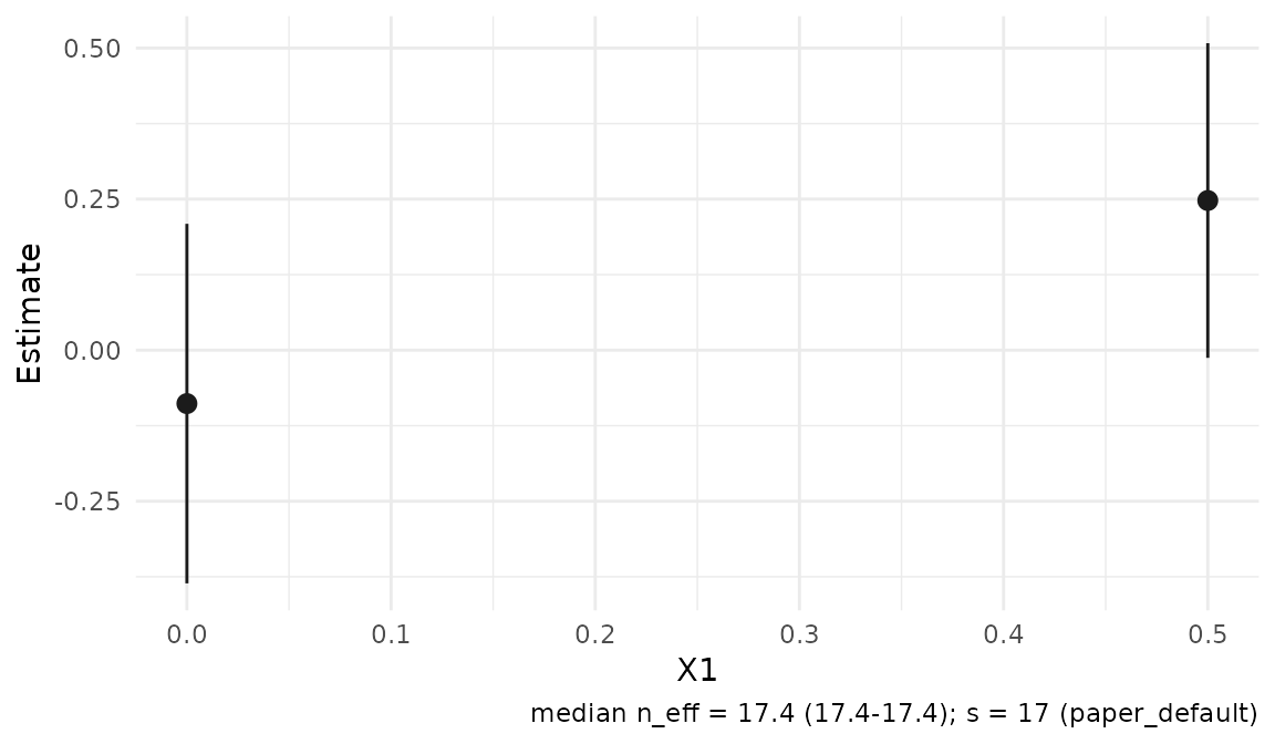

plot_weights(fit_cate, type = "profile")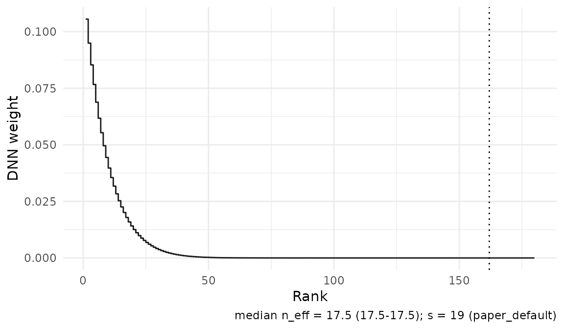

For your own scalar signal, build weights directly. Rows of W index observations and columns index target points:

wt <- weights_dnn(
  X = X, X0 = rbind(c(0, 0), c(0.5, 0)), k = 1L, s = 12L,
  return = "W"
)
dim(wt$W)
#> [1] 180   2
as.vector(crossprod(wt$W, fit_cate$psi))
#> [1] 0.562277 1.169279