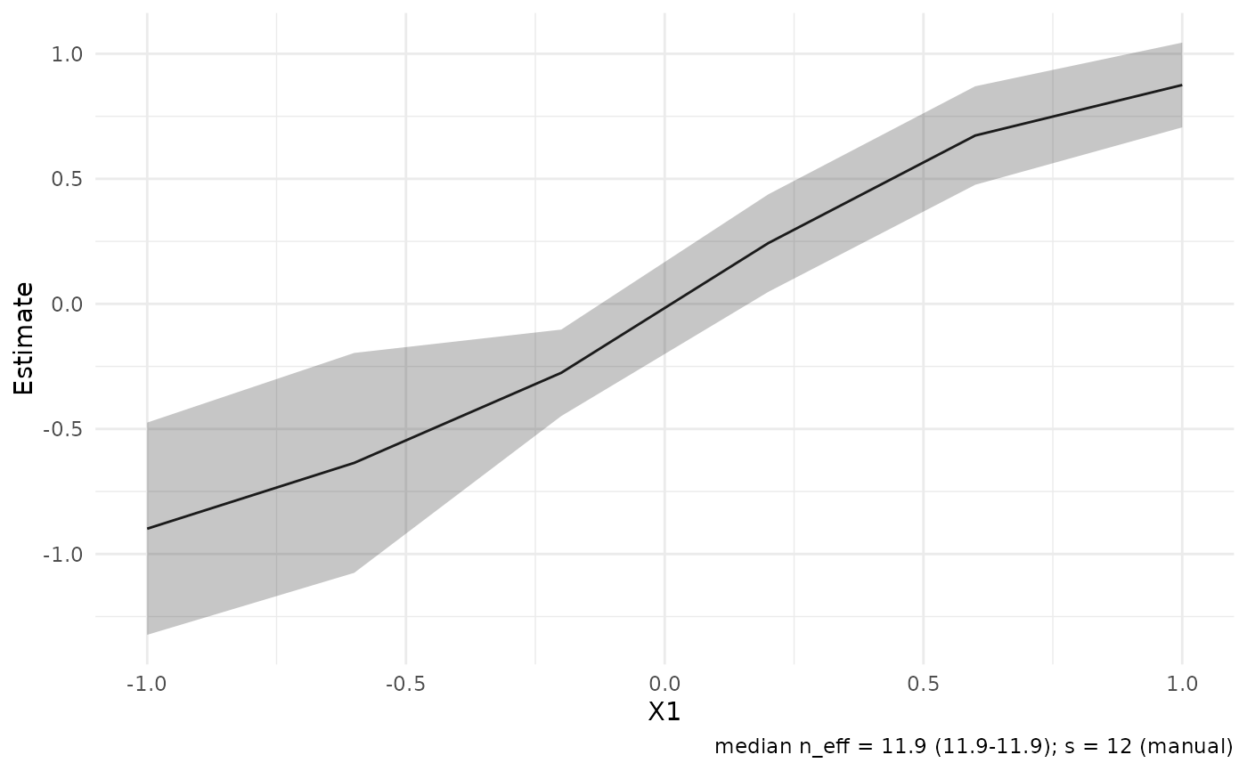
Plot estimates with confidence bounds across target points

The estimate panel of the plotting layer: point estimates with normal confidence bounds from the stored jackknife standard errors, drawn as a profile band when the targets vary along a single stored coordinate, as a forest layout for small non-profile target sets, and as pointranges otherwise. autoplot() and plot() on np_result and cate_result objects delegate here.

Usage

plot_estimates(
  object,
  level = 0.95,
  style = c("auto", "profile", "pointrange", "forest"),
  x_var = NULL,
  shade_significant = FALSE,
  candidates = "default",
  ...
)

autoplot.np_result(object, ...)

autoplot.cate_result(object, ...)

autoplot.plqr_result(object, ...)

autoplot.gmm_result(object, ...)

# S3 method for class 'np_result'
plot(x, ...)

# S3 method for class 'cate_result'
plot(x, ...)

# S3 method for class 'plqr_result'
plot(x, ...)

# S3 method for class 'gmm_result'
plot(x, ...)

Arguments

object

A fitted result object accepted by plot_data_estimates().

level

Confidence level for the bounds (default 0.95).

style

One of "auto", "profile", "pointrange", or "forest". "auto" picks a profile band when a profile axis exists and there are at least four targets, a forest layout for 2..12 non-profile targets, and pointranges otherwise.

x_var

Optional profile-axis override: a stored coordinate name (see attr(plot_data_estimates(object), "x0_names")), an x0_* column name, or a coordinate index.

shade_significant

Logical (default FALSE); for profile-style CATE panels, add a rug along the axis where the confidence interval excludes zero. Intervals are marked, never point estimates.

candidates

Candidate rows to compare for grid fits. The default "default" preserves the scalar-fit display. Use "all" or a character vector of candidate ids to compare stored grid candidates without refitting.

...

Passed to methods (for autoplot()/plot()) or ignored.

x

A fitted result object (for the plot() methods).

Value

A ggplot object.

Details

Every panel carries an honesty caption with the median effective sample size across targets (when weight diagnostics are available) and the kernel order s with its provenance (paper_default or manual). CATE panels draw a dashed zero reference line.

Experimental methods

Methods for plqr_result objects are experimental, as is all PLQR functionality in this release; see plqr_dnn().

Examples

if (requireNamespace("ggplot2", quietly = TRUE)) {
  set.seed(1)
  n <- 80
  x_mat <- matrix(rnorm(n * 2), n, 2,
                  dimnames = list(NULL, c("X1", "X2")))
  y_vec <- x_mat[, 1] + rnorm(n, sd = 0.3)
  X0 <- cbind(seq(-1, 1, length.out = 6), 0)
  fit <- np_dnn(X = x_mat, X0 = X0, Y = y_vec, k = 1L, s = 12L)
  plot_estimates(fit)
}